Constructing a timetable is hard work. But you can take quite a bit of the grunt work out of it using spreadsheets. Warning – This is a technical post, so I apologize up front. It assumes you have some basic familiarity with Google Sheets and its formulas – which, BTW are free!!
I have borrowed and adapted a technique I saw elsewhere on the web for Excel and built formulas to populate a Google spreadsheet timetable using look-aside tables. In this way, I can enter a single time for the train at its origin and the other timings will be populated automatically. Ultimately I may choose to tweak these, but at least I don’t have to add up to 20 timings to each train, and if I change that single start (or end) time everything else adjusts auto-magically. Likewise if I change my mind about how long a type of train should take to get between stations or to wait at a station. I’ve shared a sample spreadsheet on Google for my layout; this post is about how far I have got so far and how I have gone about it.
The way it works is this –
- In the first Tab of the Sheet
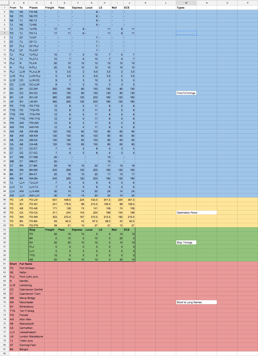
- I built a table of timings in minutes which I named as a range called “FromToTimings” where the rows are times taken between stations and are labelled with a shortened form of each name in a “from-to” format and the columns are named for each type of train I want (Passenger, Express, Local, Freight, etc). For example, Bath Green Park to Bristol would be BGP-BR. Bristol to Bath would be BR-BGP. The name choices and column choices here are arbitrary. Your going to need to enter them in the formulas, so it helps if you make them distinctive and short.
- I named the range Data->Named Ranges... of from-to row names in FromToTimings as a table “Places” and another for the column header range as “Types”.
- I built a second table in the same sheet under the first of stop/wait times at every station I showed two lines in the actual timetable (an “arr” and “dep”) with the same train type columns. I named this table as range “Stops” and the row header station names as range “StopNames”
- I built a look up table for the shortened names used in from-to and the real names (didn’t actually use this in the formulas, but its handy to look at when you have >20 stations as I have. The reason to have the short form is to shorten the length of the formulas for the timetable itself).
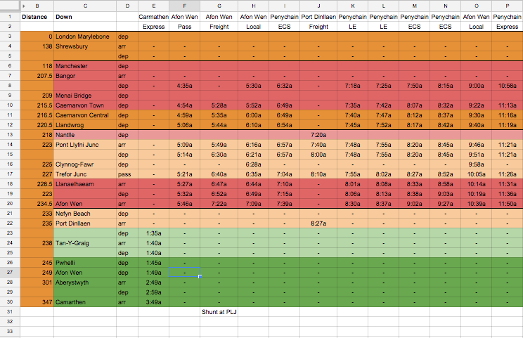
- Then I constructed UP and a DOWN tabs in classical timetable format (header rows of destination (row1) and trainType (row 2) followed by one row for each station, or two if it has both arr and depart times, the first column has station names and the second an arr/dep/pass column and then one more column for each train)
Spreadsheet Magic
- Now the magic! -> I populated each cell in a column with a formula that applies the timing values from the lookup table to the sheet based on the station to station timings and train type.
For example, a basic entry for cell “A5” will be
=IF(ISNUMBER(A4),A4+TIME(0,INDEX(FromToTimings,MATCH(Places,”From–To“,0),MATCH(Types,A$2)),0),”-“).
To walk through the formula, the “ISNUMBER” test is looking to see if there is a train at the previous station (because it will have a time if it reached there). If it does, we add the correct timing from the FromToTimings table using INDEX based on finding the name of the From–To line using MATCH on then a second MATCH to find the right column for the type of train using the type in row 2 at the top of the column. If it doesn’t have a time at the previous station, we just insert a “-“.
For station with both an arr. at “A5” and dep. at “A6” we need to add the stop/wait time instead, so the A6 cell would have =IF(ISNUMBER(A5),A5+TIME(0,INDEX(Stops,MATCH(StopNames,”To“,0),MATCH(Types,A$2)),0),”-“)
Now after routes diverge (at a junction) you need to add a little conditional logic to the basic test at the next station and look at the destination to decide if the train is coming past this station. This is the first use of the row 1 destination field.
=IF(AND(ISNUMBER(A4),A$1=”DestinationOnThisRoute“), … You can add as many destinations as you need inside the AND statement if there are many possible destinations.
For stops that can be missed out, usually the train type will need to be tested. =IF(AND(ISNUMBER(A4),A$2=”Local”), … At the next row after a missed station you’ll need to chain two IF statements, one to look at the last station as usual and if that is not satisfied another to look at the last but one. As in
=IF(ISNUMBER(A4),A4+TIME(0,INDEX(FromToTimings,MATCH(Places,”FromA4–ToA5“,0),MATCH(Types,A$2)),0),
IF(ISNUMBER(A3),A3+TIME(0,INDEX(FromToTimings,MATCH(Places,”FromA3–ToA5“,0),MATCH(Types,A$2)),0),”-“))
For converging routes, the formula will have another IF chained after the first one =IF(ISNUMBER(CellOnRoute1),TimeFromRoute1,IF(ISNUMBER(CellOnRoute2),TimefromRoute2,”-“)), …
For trains that terminate mid-route, you obviously test that the train is continuing at the next stop using
=IF(AND(ISNUMBER(A4),A$1<>”A4Name“), … Subsequent stops will then see the “-” and not add a time…
Make a copy of that column with all the formulas as a “Master column” probably on a separate tab so that even if you overwrite a cell in the latest train (to start a train from an intermediate station, for example) you have all the formulas preserved..
So that covers the basic timetable. You add a column (copy all the formulas from your master column) and plug in a destination a train type and a time at the origin – then the formulas populate all the intermediate times for a train. Woohoo!!
Extra Magic
I have found in practice, that if you a building a complex timetable that you are cobbling together from real WTTs or where you have special timings to work with, you often want to enter the time that a train arrives at a destination instead of the start. If you add formulas for that willy-nilly you’ll create circular formulas. So for this need I have constructed extra master columns in each direction for each destination that
- first back-calculates the time at the origin based on the destination time and then
- uses the same formulas as in the original master to fill out all the rest of the information for the intermediate stops.
To select the origin, I added a row at the bottom of the sheet. To simplify the formula writing I added a FromToTiming row in the timing sheet directly for each origin to destination that is calculated by adding up the timings and stops from all the stations along the route. In that way the origin cell only needs to specify one INDEX value and subtract it from the desired destination time to find the correct start time.
For example
=IF(AND(ISNUMBER(DestinationCell),A$OriginNameRow=”ThisStationName“),
DestinationCell-(TIME(0,INDEX(FromToTimings,MATCH(Places,”Origin–Destination“,0),MATCH(Types,A$2,0),0),”-“)
Note you only need to add this formula for starting stations for trains that could appear in the origin cell. If this is an intermediate station on some routes and a possible origin station on others, you can chain this origin formula inside the else part of the existing IF statement for the through train so that both a through train and a originating train are possible.
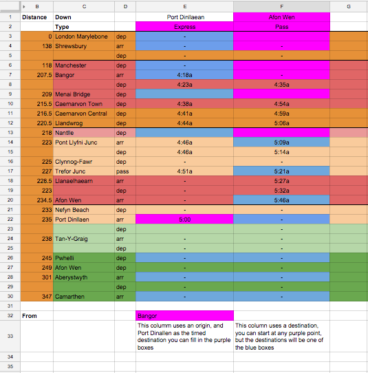
For ease of use, I color code the master to remind me where I could put in values. I used purple for entry fields and blue for the available choices of destination or origin. Once I have made copies of the column in the timetable pages and filled them in, I’ll go and reset the colors to suit the rest of the timetable.
Now copy that “destination master” column and then remember to put a plain time at the destination station, and name the starting station, you can alter the train type as well.. If there are multiple possible destinations you want to be able to code in this way, you’ll need one column each.